Analysis: FE_FE0
Key Findings and Interpretation
The regression model for the response variable FE_FE0 is statistically significant, explaining 81.43% of the total variance in the data ($R^2$). The adjusted $R^2$ of 75.46% suggests the model is robust, though the gap between the adjusted and predicted $R^2$ (53.0%) indicates some sensitivity to specific data points or potential outliers (specifically Observation 16). The analysis identifies the interaction between Magnetic Nanoparticles (MNP) and Nostoc M2 (NcM2) as the dominant factor affecting the response, exhibiting a highly significant p-value (< 0.001) and a substantial negative coefficient (-20.4).
While NcM2 individually contributes positively to the response (+0.8275), its combination with MNP creates a strong antagonistic effect, drastically reducing the FE_FE0 value. Additionally, the process variable Calcium shows a significant positive interaction with NcM2 ($p=0.011$), indicating that higher calcium levels enhance the effect of the cyanobacteria. Secondary antagonistic interactions were observed between Water and NcM2, as well as Alginate and NcM2, suggesting that formulation complexity generally hinders this specific response.
Regression Equation
The relationship between the mixture components (Water, Alg, MNP, NcM2), the process variable (Calcium), and the response FE_FE0 is described by the following regression equation. The equation includes linear mixture terms and significant interaction effects selected via stepwise regression.
Model Goodness-of-Fit
The model demonstrates a reasonably good fit to the experimental data, successfully capturing the primary drivers of variance. However, the predictive capability suggests caution when extrapolating results.
- R-sq (81.43%): Indicates that approximately 81% of the variation in FE_FE0 is explained by the model terms.
- R-sq(adj) (75.46%): adjusts for the number of predictors; the closeness to the unadjusted R-sq confirms the selected terms are meaningful.
- S (0.0936): The standard error of the regression is low, implying the data points fall relatively close to the fitted regression line.
- R-sq(pred) (53.0%): This value is notably lower than the adjusted R-sq, which often signals the presence of influential outliers (e.g., Obs 16 with a Standardized Residual of 3.91) or overfitting.
Model Summary: Stepwise Selection
The following table shows the stepwise selection process for the final model. The last row, highlighted, represents the chosen model with the best combination of explanatory and predictive power.
| Step | Term Added | R-sq (%) | R-sq(adj) (%) | S |
|---|---|---|---|---|
| 1 | Linear Terms (Water, Alg, MNP, NcM2) | 45.82 | 41.03 | 0.1450 |
| 2 | MNP*NcM2 | 64.08 | 59.72 | 0.1199 |
| 3 | Water*NcM2 | 69.55 | 64.79 | 0.1121 |
| 4 | Alg*NcM2 | 74.37 | 69.41 | 0.1045 |
| 5 | Alg*MNP | 76.44 | 70.94 | 0.1018 |
| 6 | NcM2*Calcium | 78.38 | 72.41 | 0.0992 |
| 7 | MNP*NcM2*Calcium | 81.43 | 75.46 | 0.0936 |
Model Diagnostic Plots
The diagnostic plots reveal generally acceptable model behavior, though specific outliers require attention to ensure robust predictions.
- Normality of Residuals: The Normal Probability Plot generally follows a straight line, satisfying the normality assumption, although the tails show some deviation due to outliers.
- Constant Variance: The Residuals vs. Fits plot shows a relatively random scatter, but there is a slight indication of uneven variance driven by Observation 16 (Std Resid 3.91) and Observation 27 (Std Resid -2.86). These points deviate significantly from the model predictions.
- Independence: No clear patterns or trends are visible in the Residuals vs. Order plot, suggesting the assumption of independence is met.
- Remediation: Given the high standardized residual of Obs 16, an investigation into this experimental run is recommended to rule out data entry errors or process anomalies.
Pareto Chart of Effects
In mixture designs, the standard Pareto chart of coefficients must be interpreted with caution due to the correlation inherent in the mixture constraint ($A+B+C+D=1$). While the Pareto chart visually ranks the standardized effects, highlighting the MNP*NcM2 interaction as the largest bar, it should be cross-referenced with Cox Response traces.
The Cox Response traces confirm that MNP has the steepest negative slope, indicating it is the most sensitive driver for reducing FE_FE0. Conversely, NcM2 shows a positive slope, confirming its role in increasing the response, provided it is not inhibited by the presence of MNP.
Cox Response Trace Plot
Trace plot showing the sensitivity of the response to each component relative to a reference blend.
Optimization & Prediction
The numerical optimization suggests a maximum predicted FE_FE0 response of 0.7583. This optimum is achieved at a formulation of Water (74%), Alg (1%), MNP (0%), and NcM2 (25%), with Calcium at its highest level (+1). This result aligns perfectly with the model coefficients: maximizing the positive contributor (NcM2) while completely eliminating the strong negative interactor (MNP). However, trade-offs must be considered; at this optimum, the Young's Modulus (E) is predicted to be 0.2458 and Water Content (WC) is 0.5424. If mechanical strength (E) is a critical quality attribute, this formulation might be too soft, requiring a compromise away from the absolute maximum of FE_FE0.
Calculated Optimal Conditions (Maximized FE_FE0)
0.7583
Optimal Formulation
- Water 74.0
- Alg 1.0
- MNP 0.0
- NcM2 25.0
- Calcium_Real 5
Predictions for Other Responses
- WC 0.5424
- RE 1.0417
- Ms 0.0272
- FM -0.0009
- E 0.2458
- I1 0.6116
- I2 0.528
- I3 0.4924
- I4 0.5377
- I5 0.5229
Prediction Calculator
Enter component values to predict the response for FE_FE0.
Custom Prediction
2D Contour Plots
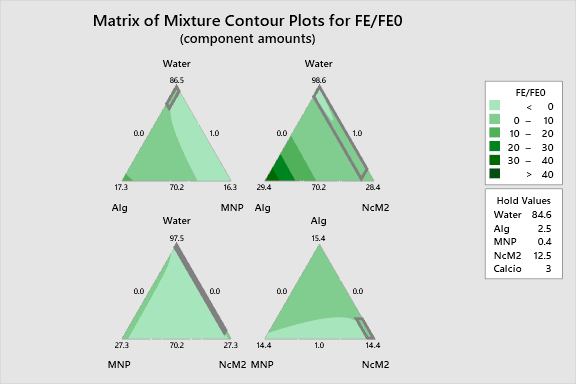
The following interactive 2D contour plots show how pairs of variables influence the response while holding the other factors at constant levels. These maps are essential for identifying optimal regions in the formulation space.
The plots distinctly visualize the antagonistic interaction between MNP and NcM2. As you move toward the region where both components are present, the contour colors shift rapidly to cool (low response) zones. The optimal "sweet spot" is located in the region characterized by high NcM2 and minimal MNP, reinforced by higher Calcium levels.
Alg Vs Mnp Fe Fe0
Alg Vs Ncm2 Fe Fe0
Mnp Vs Ncm2 Fe Fe0
3D Surface Plots
The following interactive 3D surface plots visualization provides a topographical view of the response surface. The surface exhibits a distinct saddle or valley shape depending on the axis view, driven primarily by the MNP*NcM2 interaction.
The topology shows a sharp decline (a valley) whenever MNP is introduced to a formulation containing NcM2. The highest peaks of the surface are found at the vertices corresponding to high NcM2 concentration in the absence of MNP.
3D representations of the response surface.