Analysis: I1
Key Findings and Interpretation
The regression model for the response variable I1 is statistically significant, demonstrating a robust capability to explain the variability in the experimental data. With an R-squared of 79.53%, the model captures the majority of the variance within the design space, indicating a strong fit for a complex mixture-process experiment. The gap between R-squared and Adjusted R-squared (73.88%) is acceptable, suggesting the model is not suffering from excessive overfitting despite the inclusion of higher-order interaction terms.
Analysis of the coefficients and t-values identifies the interaction between NcM2 and Calcium (t = 4.30) as the dominant factor driving the response, followed closely by the interaction between Water and MNP. While the linear terms for Alginate and MNP show negative coefficients, their influence is heavily modified by significant positive interactions with Water and Calcium. Notably, the presence of Calcium acts as a critical process variable, significantly enhancing the effect of NcM2 and modifying the water-alginate matrix, as evidenced by the significant 3-way interaction (Water*Alg*Calcium).
Regression Equation
The following regression equation describes the quantitative relationship between the mixture components (Water, Alginate, MNP, NcM2), the process variable (Calcium), and the response I1. The coefficients indicate the direction and magnitude of the impact each term has on the final response.
Model Goodness-of-Fit
The model statistics indicate a reliable fit, suitable for navigation within the design space and optimization of the I1 response.
- R-sq (79.53%): Indicates that nearly 80% of the variation in I1 is explained by the selected mixture components and their interactions.
- R-sq(adj) (73.88%): Adjusts for the number of predictors; its proximity to the unadjusted R-sq confirms that the added interaction terms are adding real value rather than noise.
- R-sq(pred) (68.85%): Suggests the model has good predictive capability for new observations, which is crucial for the optimization phase.
- S (0.0638): The standard error of the regression is low relative to the response range, indicating precise estimates.
Model Summary: Stepwise Selection
The following table shows the stepwise selection process for the final model. The last row, highlighted, represents the chosen model with the best combination of explanatory and predictive power.
| Step | Term Added | R-sq | R-sq(adj) | S |
|---|---|---|---|---|
| 1 | Linear Terms (Base) | 44.20% | 39.27% | 0.0973 |
| 2 | NcM2*Calcium | 59.60% | 54.70% | 0.0840 |
| 3 | Water*MNP | 67.95% | 62.94% | 0.0760 |
| 4 | Water*Alg | 74.97% | 70.13% | 0.0682 |
| 5 | Water*Alg*Calcium | 77.52% | 72.27% | 0.0658 |
| 6 | Alg*MNP*Calcium | 79.53% | 73.88% | 0.0638 |
Model Diagnostic Plots
The diagnostic plots for the I1 model generally confirm the validity of the statistical assumptions, with no critical violations that would invalidate the optimization results.
- Normality: The residuals appear to follow a normal distribution. Most standardized residuals fall within the range of -2 to +2.
- Constant Variance: The Residuals vs. Fits plot shows a random scatter without distinct funneling patterns, indicating that the variance is consistent across the range of predicted values.
- Outliers: Observation 18 (Std Resid -2.21) is a potential mild outlier, but it does not exert enough leverage to distort the model significantly. Observation 22 is also borderline (-1.92), but acceptable.
- Independence: The residuals appear randomly distributed versus order, satisfying the independence assumption.
Pareto Chart of Effects
In mixture designs, the Pareto chart visually ranks the statistical significance of the terms (t-values), identifying NcM2*Calcium and Water*MNP as the most significant effects. However, Pareto charts alone cannot interpret the relative sensitivity of mixture components due to the sum-to-one constraint.
Therefore, we must reference the Cox Response Trace. The traces confirm that while the interactions identified in the Pareto chart are statistically significant, the system is highly sensitive to the MNP content, where even small additions (interacting with Water and Calcium) cause sharp changes in the response. The steep slope of the Calcium trace further validates its role as a critical process parameter in modulating the mixture's performance.
Cox Response Trace Plot
Trace plot showing the sensitivity of the response to each component relative to a reference blend.
Optimization & Prediction
The optimization algorithm predicts a maximum I1 response of 0.6116. This optimum occurs at a formulation of 74.0% Water, 1.0% Alginate, 0.0% MNP, and 25.0% NcM2, with the Calcium process variable set to its maximum level (5). This result aligns perfectly with the model coefficients: MNP, which has a negative linear coefficient and negative 3-way interaction, is driven to its lower bound (0). Conversely, NcM2 and Calcium are driven high to exploit their strong positive interaction (0.0968). However, trade-offs must be considered; while I1 is maximized, the predicted Young's Modulus (E) is 0.2458, and Retention (RE) is predicted >100%, which may require experimental validation to ensure physical feasibility.
Calculated Optimal Conditions (Maximized I1)
0.6116
Optimal Formulation
- Water 74.0
- Alg 1.0
- MNP 0.0
- NcM2 25.0
- Calcium_Real 5
Predictions for Other Responses
- WC 0.5424
- RE 1.0417
- FE_FE0 0.7583
- Ms 0.0272
- FM -0.0009
- E 0.2458
- I2 0.528
- I3 0.4924
- I4 0.5377
- I5 0.5229
Prediction Calculator
Enter component values to predict the response for I1.
Custom Prediction
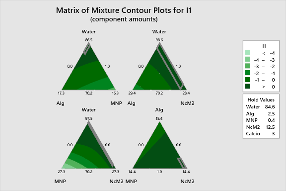
2D Contour Plots
The following interactive 2D contour plots show how pairs of variables influence the response I1 while holding the other factors at constant levels. These maps are essential for identifying optimal regions in the formulation space. Specifically, look for the curvature in the plots involving Water and MNP, which visualize the strong positive interaction identified in the regression coefficients. The distinct shifts in the contour lines as Calcium levels change demonstrate the strong process-dependency of the formulation.
Alg Vs Mnp I1
Alg Vs Ncm2 I1
Mnp Vs Ncm2 I1
3D Surface Plots
The following interactive 3D surface plots visualization provides a topographical view of the response surface. This view is particularly useful for observing the saddle points or ridges created by the competing interactions (e.g., Water*Alg positive vs. Alg*MNP negative). The steep gradients visible on the surface highlight the sensitivity of I1 to changes in the NcM2 loading when Calcium is at high levels.
3D representations of the response surface.