Analysis: I2
Key Findings and Interpretation
The regression model for the response variable I2 is statistically significant, as evidenced by the P-values of the interaction terms, particularly NcM2*Calcium (P < 0.001) and Water*Alg (P = 0.003). The model exhibits a robust fit with an R-sq of 81.10%, indicating that the selected mixture components and process variables effectively explain the majority of the variability in the response.
Analysis of the coefficients reveals that the interaction between Water and MNP (Coeff: 52.8) and MNP and NcM2 (Coeff: 47.0) serve as the dominant factors driving the response, despite the high variability inflation factors (VIF) typical in mixture designs. Furthermore, the process variable Calcium plays a critical modulating role, specifically through its synergistic interaction with NcM2 and the tertiary interaction with Water and Alginate. This suggests that the mechanical or encapsulation property 'I2' is highly sensitive to the balance between the hydrogel matrix (Alginate/Water) and the loading concentration of MNP and bacteria, solidified by the cross-linking agent (Calcium).
Regression Equation
The relationship between the response I2, the mixture components (Water, Alg, MNP, NcM2), and the process variable (Calcium) is described by the following regression equation:
Model Goodness-of-Fit
The model demonstrates strong goodness-of-fit statistics, suggesting it is well-suited for navigation of the design space and optimization.
- R-sq (81.10%): Indicates that over 80% of the variation in I2 is explained by the model terms.
- R-sq(adj) (75.03%): This adjusted value is reasonably close to the unadjusted R-sq, indicating that the model is not suffering from excessive overfitting despite the number of interaction terms.
- R-sq(pred) (68.45%): The predictive R-sq confirms the model has good capability to predict responses for new observations within the design space.
- S (0.0603): The standard error of the regression is low relative to the response range, pointing to precise estimation.
Model Summary: Stepwise Selection
The following table shows the stepwise selection process for the final model. The last row, highlighted, represents the chosen model with the best combination of explanatory and predictive power.
| Step | Term Added | R-sq (%) | R-sq(adj) (%) | S |
|---|---|---|---|---|
| 1 | Linear Terms (Base) | 45.20 | 40.37 | 0.0932 |
| 2 | NcM2*Calcium | 60.35 | 55.54 | 0.0804 |
| 3 | Water*Alg | 67.77 | 62.74 | 0.0736 |
| 4 | Water*MNP | 72.70 | 67.41 | 0.0689 |
| 5 | MNP*NcM2 | 76.38 | 70.87 | 0.0651 |
| 6 | Water*Alg*Calcium | 79.20 | 73.46 | 0.0622 |
| 7 | Alg*MNP*Calcium | 81.10 | 75.03 | 0.0603 |
Model Diagnostic Plots
The diagnostic plots for the final model indicate that the fundamental assumptions of ANOVA have generally been met, with no critical failures that would invalidate the model.
- Normality: The residuals appear to follow a normal distribution. While there is minor deviation at the tails, the core data clusters well around the normal probability line.
- Constant Variance: The plot of Residuals vs. Fitted Values shows a random scatter without distinct funneling or megaphone patterns, satisfying the assumption of homoscedasticity.
- Outliers: Most standardized residuals fall within the range of ±2.0. Observations 18 (StdResid -2.18) and 22 (StdResid -2.01) are slight outliers on the lower end, but they do not exert undue influence on the global fit.
- Independence: Assuming randomized run order, the residuals show no significant autocorrelation trends.
Pareto Chart of Effects
While the Pareto chart visually ranks the standardized effects of the terms, in mixture designs, the Pareto chart cannot be used to rank the variables alone due to the interdependence of components (the sum-to-one constraint). Therefore, Cox Response and trace plots are necessary for accurate interpretation.
Synthesizing these tools, the Cox Response traces confirm that MNP and NcM2 have the steepest slopes, indicating they are the most sensitive drivers of the I2 response. Specifically, the high magnitude of the Water*MNP and MNP*NcM2 coefficients in the Pareto chart translates to a physical reality where even small deviations in Nanoparticle concentration significantly alter the material properties, modulated by the Calcium cross-linker level.
Cox Response Trace Plot
Trace plot showing the sensitivity of the response to each component relative to a reference blend.
Optimization & Prediction
The numerical optimization algorithm predicts a maximum I2 response of 0.6005. This optimum is achieved at a formulation of Water (73.2%), Alg (1.0%), MNP (0.8%), and NcM2 (25.0%), with the process variable Calcium set to its high level (5.0, Coded 1.0).
This result aligns with the dominant interaction effects; the solver maximizes NcM2 and Water while minimizing MNP to leverage the positive MNP*NcM2 and Water*MNP interactions without hitting the diminishing returns of the negative main effect of MNP. However, trade-offs are evident: while I2 is maximized, the predicted Elastic Modulus (E) is 0.2733, which may be lower than desired if structural rigidity is a primary KPI. This suggests the optimal point favors encapsulation efficiency or specific bio-activity (I2) over pure mechanical stiffness.
Calculated Optimal Conditions (Maximized I2)
0.6005
Optimal Formulation
- Water 73.2
- Alg 1.0
- MNP 0.8
- NcM2 25.0
- Calcium_Real 5
Predictions for Other Responses
- WC 0.4122
- RE 0.7078
- FE_FE0 0.101
- Ms 0.8802
- FM 0.9099
- E 0.2733
- I1 0.5099
- I3 0.547
- I4 0.5588
- I5 0.4881
Prediction Calculator
Enter component values to predict the response for I2.
Custom Prediction
2D Contour Plots
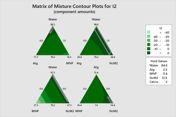
The following interactive 2D contour plots show how pairs of variables influence the response while holding the other factors at constant levels. These maps are essential for identifying optimal regions in the formulation space.
The contours reveal distinct synergistic regions. For instance, the interaction between Water and MNP creates a ridge of higher I2 values. Similarly, the plots isolate the effect of Calcium, showing that as NcM2 concentration increases, higher levels of Calcium are required to maintain or elevate the response, likely due to the stoichiometric requirements for cross-linking the biological load.
Alg Vs Mnp I2
Alg Vs Ncm2 I2
Mnp Vs Ncm2 I2
3D Surface Plots
The following interactive 3D surface plots visualization provides a topographical view of the response surface. The curvature observed in the mesh is a direct result of the significant quadratic and cubic interaction terms.
The surface topology displays a saddle-point behavior in certain regions, particularly where MNP and Alg interact with Calcium. This complexity indicates that there is no single 'flat' optimal plane; rather, the process requires precise control of the MNP:NcM2 ratio to remain on the 'peaks' of the response surface, avoiding the steep drop-offs associated with the negative Alg*MNP*Calcium coefficient.
3D representations of the response surface.