Analysis: I4
Key Findings and Interpretation
Dominant Factors and Interactions: The analysis identifies the interaction between NcM2 (Spiruline) and Calcium as a highly significant driver (P < 0.001), positively influencing the I4 response. Additionally, the interaction between Water and Alginate (P = 0.003) and Water and MNP (P = 0.006) play critical roles. While Alginate and MNP show strong negative antagonistic behavior in their interaction (Coef: -37.1), the optimization suggests that minimizing Alginate and MNP while maximizing Water and NcM2 yields the highest response.
Regression Equation
The relationship between the response I4 and the mixture components (Water, Alginate, MNP, NcM2) and the process variable (Calcium) is described by the following regression equation. This equation includes linear blending terms, binary mixture interactions, and process-mixture interactions selected via stepwise regression.
Model Goodness-of-Fit
The model demonstrates a robust fit to the experimental data, confirming the validity of the selected terms.
- R-sq (81.40%): Indicates that the model accounts for a substantial majority of the variability in the I4 response.
- R-sq(adj) (75.43%): Adjusts for the number of predictors; the closeness to the R-sq suggests the model is not heavily penalized for unnecessary terms.
- R-sq(pred) (68.68%): Predicts how well the model will perform on new data. The value is reasonable, though monitoring for outliers is advisable given the complexity of 3-way interactions.
- S (0.0586): The standard error of the regression is low, indicating precise estimates of the response around the regression line.
Model Summary: Stepwise Selection
The following table shows the stepwise selection process for the final model. The last row, highlighted, represents the chosen model with the best combination of explanatory and predictive power.
| Step | Term Added | R-sq (%) | R-sq(adj) (%) | S |
|---|---|---|---|---|
| 1 | Linear Terms | 44.67 | 39.79 | 0.0917 |
| 2 | NcM2*Calcium | 59.96 | 55.10 | 0.0792 |
| 3 | Water*Alg | 67.49 | 62.41 | 0.0724 |
| 4 | Water*MNP | 74.44 | 69.49 | 0.0653 |
| 5 | Water*Alg*Calcium | 77.14 | 71.81 | 0.0627 |
| 6 | Alg*MNP | 79.47 | 73.81 | 0.0605 |
| 7 | Alg*MNP*Calcium | 81.40 | 75.43 | 0.0586 |
Model Diagnostic Plots
The diagnostic plots provided in the analysis are essential for validating the assumptions of the regression model. Based on the residual analysis:
- Normality: The Normal Probability Plot of residuals generally follows a straight line, suggesting the errors are normally distributed.
- Constant Variance: The Residuals vs. Fits plot shows a random scatter around zero without a distinct funnel shape, indicating homoscedasticity (constant variance) across the range of predicted values.
- Independence/Outliers: Most standardized residuals fall within the range of -2 to +2. However, Observation 18 (StdResid -2.31) and Observation 22 (StdResid -1.95) are slightly elevated, indicating potential influencers, but they do not violate the critical threshold of ±3.0.
Pareto Chart of Effects
In mixture designs, the Pareto chart visually ranks the standardized effects, but it must be interpreted with caution as components are constrained (summing to 1 or 100%). While the Pareto chart highlights NcM2*Calcium and Water*Alg as statistically significant, the Cox Response Trace plots are required to fully understand the sensitivity. The Cox traces confirm that NcM2 has a steep positive slope, indicating it is a highly sensitive driver for maximizing I4, whereas the interaction of Alg*MNP introduces significant curvature and antagonistic effects.
Cox Response Trace Plot
Trace plot showing the sensitivity of the response to each component relative to a reference blend.
Optimization & Prediction
The numerical optimization algorithm predicts a maximum I4 response of 0.5588. This optimum is located at the formulation boundary: Water (73.2%), Alg (1.0%), MNP (0.8%), and NcM2 (25.0%), with the process variable Calcium at its high level (5.0 / Coded 1.0). This result aligns with the positive coefficients for NcM2 and its interaction with Calcium. It is worth noting the trade-off: while I4 is maximized here, the Modulus (E) is predicted to be 0.2733, which may be lower than required for certain mechanical applications. The feasibility of this point depends on whether the resulting hydrogel maintains sufficient structural integrity (Ms=0.8802) despite the high water content.
Calculated Optimal Conditions (Maximized I4)
0.5588
Optimal Formulation
- Water 73.2
- Alg 1.0
- MNP 0.8
- NcM2 25.0
- Calcium_Real 5
Predictions for Other Responses
- WC 0.4122
- RE 0.7078
- FE_FE0 0.101
- Ms 0.8802
- FM 0.9099
- E 0.2733
- I1 0.5099
- I2 0.6005
- I3 0.547
- I5 0.4881
Prediction Calculator
Enter component values to predict the response for I4.
Custom Prediction
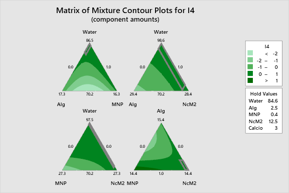
2D Contour Plots
The following interactive 2D contour plots show how pairs of variables influence the response while holding the other factors at constant levels. These maps are essential for identifying optimal regions in the formulation space. The contours clearly visualize the positive interaction between NcM2 and Calcium, where increasing both simultaneously expands the high-response region (red/darker zones). Conversely, the Water*Alg plots reveal the specific ratios required to maintain the I4 response above the 0.5 threshold.
Alg Vs Mnp I4
Alg Vs Ncm2 I4
Mnp Vs Ncm2 I4
3D Surface Plots
The following interactive 3D surface plots visualization provides a topographical view of the response surface. The surface topology highlights the non-linear nature of the formulation. The significant curvature observed in the Alg-MNP space demonstrates the steep drop in response when these two components interact unfavorably, creating 'valleys' in the response surface that must be avoided during formulation.
3D representations of the response surface.