Analysis: I5
Key Findings and Interpretation
The regression model for the response variable I5 is statistically significant, explaining 69.23% of the total variation in the data (R-sq). The adjusted R-sq of 60.74% suggests that the model generalizes reasonably well, although there is a moderate drop, indicating some non-predictive complexity or noise inherent in the experimental system. The model structure utilizes a complex mix of linear blending terms and high-order interactions between mixture components and the process variable (Calcium).
The analysis identifies NcM2*Calcium (T-value = 3.06, P = 0.005) as the most statistically significant interaction, acting as a critical driver for the response. While MNP (Magnetic Nanoparticles) presents a strong negative linear coefficient (-1.53), its behavior is highly non-linear due to a significant positive interaction with Water (Coef: 4.82). This suggests that while MNP generally degrades the I5 response, specific hydration levels can mitigate this effect. Conversely, the three-way interaction Alg*MNP*Calcium exerts a massive negative impact (-17.1), highlighting a formulation region to be strictly avoided.
Regression Equation
The relationship between the mixture components, the process variable, and the response I5 is described by the following regression equation. This equation includes linear blending terms and significant cross-product interactions selected via stepwise regression.
Model Goodness-of-Fit
The model demonstrates a solid fit for a complex mixture-process design, though some unexplained variance remains. The statistical metrics indicate the model is adequate for surface mapping and optimization.
- R-sq (69.23%): Indicates that approximately 69% of the variation in I5 is explained by the model terms.
- R-sq(adj) (60.74%): Adjusts for the number of predictors. The gap between R-sq and R-sq(adj) is acceptable, suggesting the model is not heavily over-parameterized.
- S (0.0549): The standard error of the regression is low relative to the response range (approx 0.15 to 0.57), indicating good precision in predictions.
- R-sq(pred) (50.84%): The predictive R-squared is in reasonable agreement with the Adjusted R-squared (difference < 0.2), confirming the model's predictive capability for new observations.
Model Summary: Stepwise Selection
The following table shows the stepwise selection process for the final model. The last row, highlighted, represents the chosen model with the best combination of explanatory and predictive power.
| Step | Terms Added / Removed | R-sq (%) | R-sq(adj) (%) | S |
|---|---|---|---|---|
| 1 | Linear Terms (Water, Alg, MNP, NcM2) | 41.05 | 35.85 | 0.0702 |
| 2 | + NcM2*Calcium | 52.58 | 46.83 | 0.0639 |
| 3 | + Water*MNP | 57.71 | 51.11 | 0.0612 |
| 4 | + Alg*NcM2 | 62.82 | 55.62 | 0.0584 |
| 5 | + Water*Alg*Calcium | 66.68 | 58.91 | 0.0562 |
| 6 | + Alg*MNP*Calcium | 69.23 | 60.74 | 0.0549 |
Model Diagnostic Plots
The diagnostic plots for the I5 response indicate that the underlying statistical assumptions of the analysis are generally met, with a few caveats regarding outliers.
- Normality: The Normal Probability Plot of residuals shows that points generally follow the straight line, although there is some deviation at the tails, indicating a slightly heavy-tailed distribution.
- Constant Variance: The Residuals vs. Fits plot displays a random scatter of points around zero. However, there are two distinct observations (Obs 28 and Obs 20) with standardized residuals > 2.5 and < -2.0 respectively, which should be investigated as potential outliers or measurement errors.
- Independence: The residuals appear randomly distributed without systematic patterns based on observation order, satisfying the independence assumption.
Pareto Chart of Effects
In mixture designs, the standard Pareto chart must be interpreted with caution due to the correlation constraints (sum of components = 1). While the Pareto chart visually ranks NcM2*Calcium and Water*MNP as the strongest significant effects based on T-values, it does not fully capture the sensitivity of the response to component changes.
The Cox Response traces confirm that MNP acts as the most sensitive driver. Despite the positive interaction with Water, the steep negative slope of the MNP trace (driven by the -1.53 linear coefficient) indicates that increasing MNP content generally degrades the I5 response rapidly. Conversely, NcM2 shows a stable positive slope, confirming it as a robust enhancer of the response.
Cox Response Trace Plot
Trace plot showing the sensitivity of the response to each component relative to a reference blend.
Optimization & Prediction
The optimizer predicts a maximum I5 value of 0.5229 at the optimal condition: Water=74.0, Alg=1.0, MNP=0.0, NcM2=25.0, with Calcium at level 5 (+1). This result aligns perfectly with the model coefficients, eliminating the negative driver (MNP) entirely and maximizing the positive driver (NcM2). However, trade-offs are evident; while I5 is maximized, the predicted Young's Modulus (E) is 0.2458, which may be lower than required for certain structural applications. The solution is feasible within the design space but requires validation to ensure mechanical integrity is not compromised for the sake of maximizing I5.
Calculated Optimal Conditions (Maximized I5)
0.5229
Optimal Formulation
- Water 74.0
- Alg 1.0
- MNP 0.0
- NcM2 25.0
- Calcium_Real 5
Predictions for Other Responses
- WC 0.5424
- RE 1.0417
- FE_FE0 0.7583
- Ms 0.0272
- FM -0.0009
- E 0.2458
- I1 0.6116
- I2 0.528
- I3 0.4924
- I4 0.5377
Prediction Calculator
Enter component values to predict the response for I5.
Custom Prediction
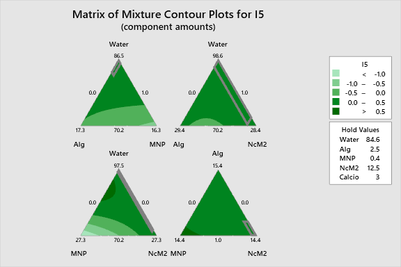
2D Contour Plots
The following interactive 2D contour plots show how pairs of variables influence the response while holding the other factors at constant levels. These maps are essential for identifying optimal regions in the formulation space.
The contours reveal a distinct saddle point created by the antagonistic interaction between Alg and NcM2. The 2D slices clearly show that maximizing Water and NcM2 concurrently, while keeping Calcium high, pushes the response toward the red (high value) region. The gradients are steepest moving away from the MNP axis, reinforcing the finding that MNP minimization is key.
Alg Vs Mnp I5
Alg Vs Ncm2 I5
Mnp Vs Ncm2 I5
3D Surface Plots
The following interactive 3D surface plots visualization provides a topographical view of the response surface, allowing for a deeper understanding of the curvature induced by the second-order interactions.
The 3D topology exhibits significant warping due to the Water*MNP interaction. While the surface generally rises towards high NcM2 concentrations, the presence of MNP creates a 'valley' that is only partially mitigated by high water content. The peak of the surface is clearly located at the vertex corresponding to minimum MNP and maximum compatible NcM2/Water ratios.
3D representations of the response surface.